Examples

A complete analysis of a small artificial data set: four trees on eight taxa, as from a small posterior sample, with taxon costs and survival probabilities. Each output shown is produced by the code above it. The last section applies the same steps to data in files.

Data and structure

Data

The four trees share the split between \(\{A, B, C, D\}\) and \(\{E, F, G, H\}\) and differ within each half. The weights are posterior frequencies; the costs and survival probabilities are per taxon.

>>> import forestpd as fpd
>>> trees = [
...     "((A:2,B:3):4,(C:1,D:5):2,((E:3,F:2):1,(G:4,H:1):3):2);",
...     "((A:2,C:3):4,(B:1,D:5):2,((E:3,F:2):1,(G:4,H:1):3):2);",
...     "((A:2,B:3):4,(C:1,D:5):2,((E:3,G:2):1,(F:4,H:1):3):2);",
...     "((A:2,D:3):3,(B:1,C:5):3,((E:3,F:2):1,(G:4,H:1):3):2);",
... ]
>>> weights = [0.4, 0.3, 0.2, 0.1]
>>> costs = {"A": 2, "B": 1, "C": 3, "D": 1, "E": 2, "F": 4, "G": 1, "H": 2}
>>> survival = {"A": 0.9, "B": 0.2, "C": 0.5, "D": 0.1, "E": 0.6, "F": 0.3, "G": 0.05, "H": 0.7}
>>> instance = fpd.MaxMPDInstance(trees, costs=costs, weights=weights, survival=survival)

Instance structure

structure() reports the clusters and agreement-forest sizes without solving:

>>> structure = instance.structure()
>>> structure.n_clusters, structure.maf_sizes, structure.n_signatures
(2, (2, 3), 16)

The shared split divides the instance into two clusters, one per half, with agreement forests of 2 and 3 components: 16 signatures in total. Larger data sets have thousands of clusters, and the largest \(k\) determines the running time.

Budget curve

Optimal sets per budget

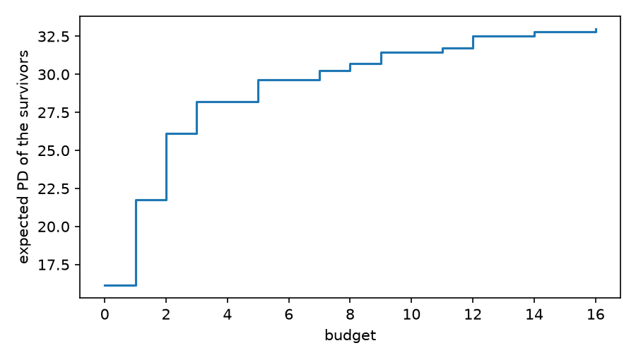
optimize_many() over all budgets from 0 to the total cost gives the optimum and an optimal set for each:

>>> total = sum(costs.values())
>>> results = instance.optimize_many(range(total + 1), return_taxa=True)
>>> for budget in (0, 1, 2, 8, 10, 12, 16):
...     print(budget, round(results[budget].value, 2), sorted(results[budget].taxa))
0 16.14 []
1 21.76 ['D']
2 26.14 ['D', 'G']
8 30.69 ['B', 'C', 'D', 'E', 'G']
10 31.44 ['B', 'D', 'E', 'F', 'G']
12 32.5 ['B', 'C', 'D', 'E', 'F', 'G']
16 33.0 ['A', 'B', 'C', 'D', 'E', 'F', 'G', 'H']

With nothing protected, the expected PD is 16.14, since unprotected taxa may survive. D and G, both cheap and at high risk, add 10 of the 16.86 that protection can add. The optimal sets are not nested: C is in the optimal set at budget 8, not at 10, and again at 12. A ranking of individual taxa cannot give such sets.

Plotting the curve

import matplotlib.pyplot as plt

plt.step(range(total + 1), [r.value for r in results], where="post")
plt.xlabel("budget")
plt.ylabel("expected PD of the survivors")
plt.show()

Comparison with simpler plans

Planning on one tree

The set that is optimal on the first (most probable) tree alone, scored on all four trees. Survival probabilities are left out here, so that only the trees differ:

>>> all_trees = fpd.MaxMPDInstance(trees, costs=costs, weights=weights)
>>> tree_1 = fpd.MaxMPDInstance(trees[:1], costs=costs)
>>> best = all_trees.optimize(6, return_taxa=True)
>>> plan = tree_1.optimize(6, return_taxa=True).taxa
>>> sorted(best.taxa), best.value
(['A', 'D', 'E', 'G'], 24.5)
>>> sorted(plan), all_trees.evaluate_pd(plan)
(['B', 'D', 'E', 'G'], 23.8)

On the first tree, B adds more than A next to D, E and G (7 against 6: its own branch and the edge above it). In the second tree, B is D’s sister and adds only its own branch, of length 1, so over all four trees A adds more (5.6 against 4.9, weighted).

Ignoring extinction risk

The set that is optimal without survival probabilities, scored on the expected PD of the survivors:

>>> aware = instance.optimize(6, return_taxa=True)
>>> blind = all_trees.optimize(6, return_taxa=True).taxa
>>> sorted(aware.taxa), round(aware.value, 2)
(['B', 'D', 'E', 'G'], 29.63)
>>> sorted(blind), round(instance.evaluate_pd(blind), 2)
(['A', 'D', 'E', 'G'], 28.01)

The set chosen without survival probabilities spends 2 on A, which survives unprotected with probability 0.9. The optimal set protects B instead, which survives unprotected with probability 0.2.

Data from files

The same steps for trees in a Newick file (here a posterior sample) and a CSV file with a cost (an integer of at least 1) and a survival probability per species:

import csv

import forestpd as fpd

with open("species.csv") as handle:   # columns: species, cost, survival
    rows = list(csv.DictReader(handle))
costs = {row["species"]: int(row["cost"]) for row in rows}
survival = {row["species"]: float(row["survival"]) for row in rows}

instance = fpd.MaxMPDInstance("posterior.nwk", costs=costs, survival=survival)
print(instance.structure())
for budget, result in enumerate(instance.optimize_many(range(201), return_taxa=True)):
    print(budget, result.value, sorted(result.taxa))

Every tree has weight 1 here, so the values are sums over the trees; with weights=[1 / t] * t they are means, with the same optimal sets.

For larger or more discordant tree sets, install maffe and pass maf=TieredMAF() to structure() and optimize_many() (see Agreement-forest stages). For gene trees with outgroups or extra accessions, prune first (see Pruning trees to a taxon set).